 As part of a series of articles on Chaos Theory and classical programs from my early days of computing, I am sharing a favorite program which generates a population bifurcation diagram when running.
Years ago I wrote a program to generate these diagrams on my old Radio Shack Color Computer when I had a lot more black hairs on my head than I do now.
The program I will share runs on the Color Computer (both vintage COCO machines or Emulators) and is an adaptation of another author’s code. It is very similar to my original program from the 1980s. The diagram that the COCO generates is nowhere near as high quality as the images one can get with a modern graphical PC card running a full power but the program does allow a programmer to quickly and easily explore the code and play around with the variables to probe the logic and see what works or doesn’t.
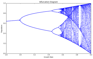
The diagram shows a growth rate in the X-dimension of the graph in relation to the population numbers on the Y-dimension. As the rate of growth is pushed higher and higher the population numbers begin to fluctuate wildly as the rate of change increases.
Before I share the program, a little education is in order as to what the formula that generates this diagram signifies and it’s importance to Chaos Theory.
The Logistic Difference Equation
The formula which drives the model is the logistic difference equation. The formula is shown below:
Xn+1 = rxn(1 – xn)
As with many fractal and chaos formulas, the output of a formula can be fed into the input of the formula which is a job uniquely suited to computers to reveal unsuspected structure and beauty once graphed on a computer display.
The formula was originally conceived to predict rise and fall in populations depending on external pressures or drivers that cause the species to thrive or fall in relation to the food available in terms of vegetation or prey animals depending on the species being looked at.
The term “r” equals the driving parameter, the factor that causes the population to change. xn represents the population of the species. To use the equation, one starts with a fixed value of r and an initial value of x. Then you run the equation iteratively to obtain values of x1, x2, x3, all the way up to xn.
A mathematical biologist named Robert May began noticing issues when he began pushing this equation beyond normal expectations and ultimately he consulted with his friend, James Yorke. Yorke who was a professor of mathematics at the University of Maryland.
Yorke was familiar with weather scientist Ed Lorenz‘s paper “Deterministic Nonperiodic Flow” in the Journal of the Atmospheric Sciences. Lorenz noted that simple equations that modeled weather systems were sensitive to the initial conditions fed to the equations and which ultimately proved that long term weather forecasts were impossible given the state of our technology. In fact we may NEVER be able to predict weather with any precision.
Yorke was of the belief that there might be a similar behavior between the equations Lorenz used for his weather models and the animal population model May was working with. Yorke then took the logistic difference equation and ran it through its paces.
Yorke began with low values of r, just as May had, then kept pushing the value higher and higher. As long as r remained below 3.0, xn converged to a single value. But when setting r equal to 3.0, xn oscillated between two values. On a map or diagram, this appeared as a single line dividing into two branches — a bifurcation.
Yorke kept moving the value of r even higher. As this increased, xn experienced additional bifurcations, oscillating between four values, then eight, then sixteen. When the driving parameter equaled 3.569945672, xn neither converged nor oscillated — it became completely random. And when r hit values greater than 3.569945672, xn exhibited complete randomness punctuated by “windows” of stability.
Yorke and co-author T.Y. Li summarized their findings in “Period Three Implies Chaos,” a 1975 landmark paper that introduced the world to the term “chaos” and “chaotic” behavior. Yorke reaffirmed and popularized what prior Chaos Science explorers Henri Poincaré and Ed Lorenz had already discovered as early as the 19th century: The fact is that simple theoretical and real-world systems could be and are governed by relatively simple equations.
Henri Poincaré was there ahead of all others and remarkably predicted that the Universe is far more sensitive to everything within it than otherwise would be imagined. The clockwork certainty of Newtonian Physics was doomed at this realization although many had not yet realized it. The Universe is not all all the orderly place one would reason it to be and for which Science had placed so much stock in. Poincaré described the Hallmark term of Chaos – sensitive dependence on initial conditions. The term received he coined received relatively little notice until the late 20th Century when Chaos Science began to hit the mainstream. In Poincaré’s own words:
If we knew exactly the laws of nature and the situation of the universe at the initial moment, we could predict exactly the situation of that same universe at a succeeding moment. but even if it were the case that the natural laws had no longer any secret for us, we could still only know the initial situation approximately. If that enabled us to predict the succeeding situation with the same approximation, that is all we require, and we should say that the phenomenon had been predicted, that it is governed by laws. But it is not always so; it may happen that small differences in the initial conditions produce very great ones in the final phenomena. A small error in the former will produce an enormous error in the latter. Prediction becomes impossible, and we have the fortuitous phenomenon. – in a 1903 essay “Science and Method”
Chaos equations produce complex and often unpredictable behavior that the unsuspecting person might miss at first glance unless iterating the formula through a computer model. The models not only produce a window into the chaos that can unfold into systems like populations or weather but also reveal windows of order that arise as more and more energy or change is introduced into a system.
The Color Computer Program
I modified this program based on one found at Michael Logusz’s web site which was remarkably easy to adapt over to the COCO. Running the program takes some time because of the intensive computing going on but it is rewarding to slowly watch the bifurcation diagram emerge and to appreciate what is happening when executing the program. The diagram will take about 5 to 10 minutes to fully execute depending on your machine and is not an instant gratification sort of product to work with. That adds to it’s charm from my point of view.
While the COCO is not able to produce a detailed view like high quality modern graphics, one can appreciate that the COCO can do a “good enough” job of allowing a decent bifurcation diagram to emerge from executing the code as seen below:

The output of the Color Computer adaptation of the Bifurcation program
Program Listing
5 REM BIFURCATION PROGRAM – LOGISTIC DIFFERENCE EQUATION
7 REM SET UP THE GRAPHICS. PROGRAM MODIFIED FROM ORIGINAL SHARED AT
8 REM https://michaellogusz.blogspot.com/2018/12/basic-programming-last-time-i-played.html
10 PMODE 0,1
15 PCLS
20 SCREEN 1,1
40 COLUMNS = 255
50 ROWS = 191
55 REM CHOOSE THE START AND END POINTS FOR THE PROGRAM RUN
60 START = 1
70 FINISH = 3.999
80 TP = 0
90 BOTTOM = 1
100 MAXREPS = 10
110 HEIGHT = BOTTOM – TP
120 VPCT = 1/HEIGHT
130 FOR R = START TO FINISH STEP(FINISH – START)/COLUMNS
140 X = .1
150 FOR I = 1 TO 100
160 X = R * (X – X * X)
170 NEXT I
180 FOR I = 1 TO 30
190 X = R * (X – X * X)
200 PSET ((R-START) * COLUMNS/(FINISH-START), ROWS-(X-TP) * ROWS * VPCT,1)
210 NEXT I
220 NEXT R
300 GOTO 300
Running the program
 As most people do not own a working vintage Color Computer, the VCC Color Computer Emulator will suffice and is, more importantly, FREE.
This software emulates all types of Color Computer systems and comes with built-in BASIC to allow one to run original Radio Shack software or create their own from scratch. The software emulates all manner of varieties and peripherals that the COCO supported during it’s heyday.
Scrape and then paste the code into the VCC emulator and then type “RUN” to execute the code. I recommend you get a cup of coffee and return to slowly watch the art emerge as the formula iterates and feeds into itself over time.
Enjoy the code and I hope this inspires you to use simple retro systems like the Color Computer to explore math and science concepts. — Jon